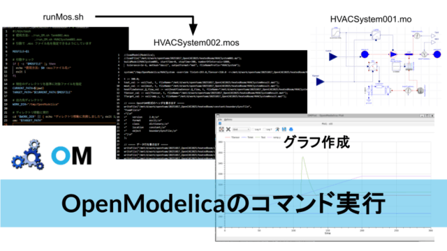
【第1回】OpenFOAMで平板流れ解析!乱流モデルと壁関数を検証
こんにちは(@t_kun_kamakiri)
乱流モデルと壁関数の選択が解析結果に大きな影響を与えることをご存知でしょうか?
本記事では、乱流モデルと壁関数の違いを理解し、それをシミュレーションで確かめるためのモデルを構築する手順をご紹介します。
オープンソース流体解析ツールとしてはOpenFOAM利用し、初心者の方でもわかりやすいように、基本から丁寧に解説していきます。この記事を通じて、乱流解析における選択の重要性を深く理解し、実践的なスキルを身につけていきましょう。
- 平板流れの解析の設定方法
- 結果出力の方法(Pythonを使用)
WSLのUbuntu 22.04.05 LTS(OpenFOAM2406)
Python 3.11.9
壁関数に関して
壁関数に関する前提知識が必要になります。
詳しい内容は記事を読んでいただければ思います。
本記事では壁関数と$y^+$に関すると最低限の内容だけを記載しておきます。
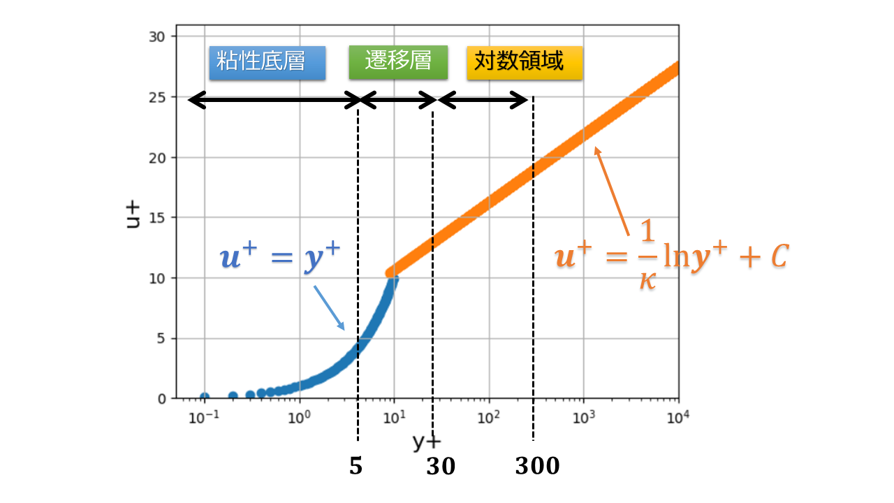
壁関数の速度分布
乱流状態では速度の乱れに応じたレイノルズ応力が発生するため、理論的に解析することが難しいのですが、実験結果に基づく経験的な解析によって壁近傍での乱流の速度分布を求めることができます。
平行平板の壁近傍の流れの漫画絵を描きました。
- 横軸:$x$方向
- 縦軸:$y$方向
壁と水平な方向($x$方向)の流速を$u$とします。
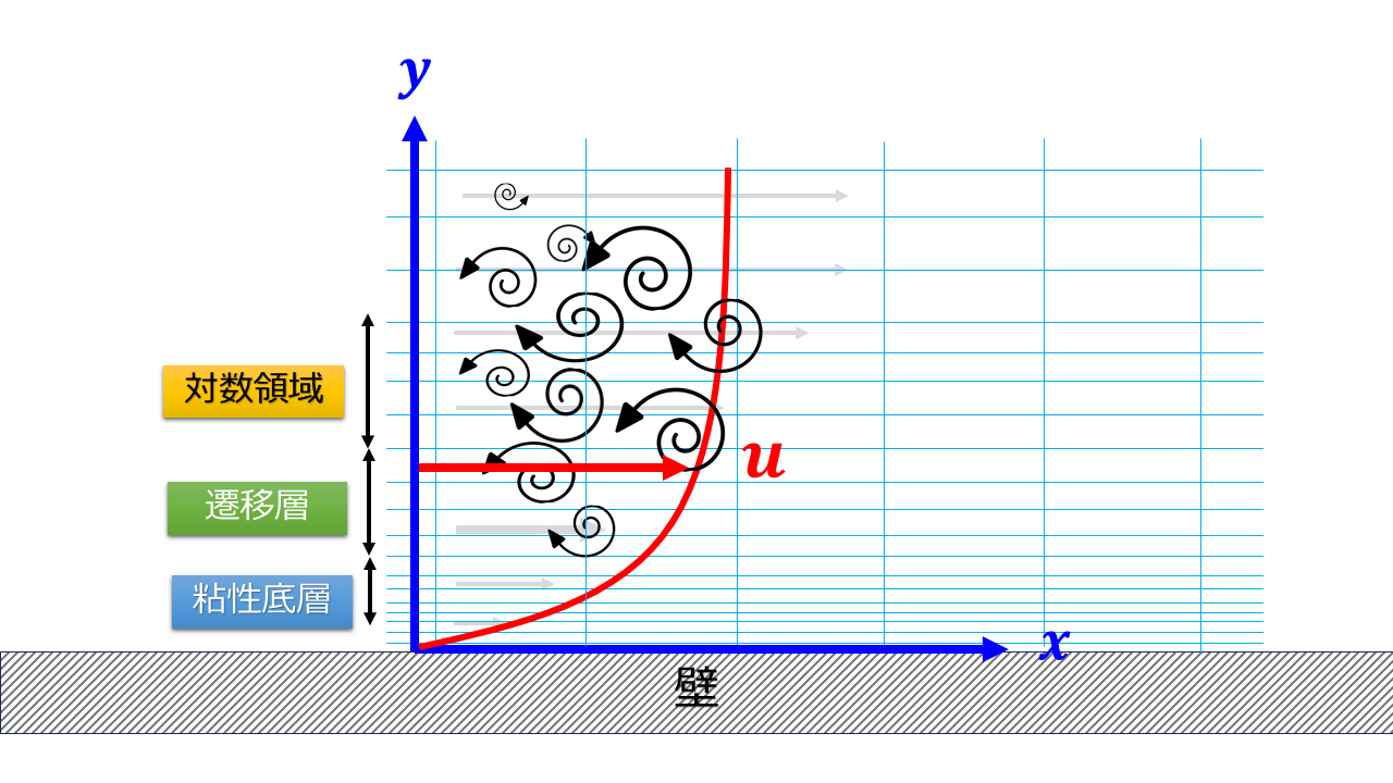 壁からの距離$y$を横軸に、壁と水平方向($x$方向)の流速$u$を縦軸にとったグラフを書くと以下のような分布になることが実験的にも確認されています。
 まずはこの分布の形を覚えましょう!
ただし、この分布の横軸と縦軸はそれぞれ以下のように壁近傍の特徴的な大きさで無次元化されていることに注意が必要です。
- $y^{+}=\frac{u_{\tau}y}{\nu}$
- $u^{+}=\frac{u}{u^{\tau}}$
※$u_{\tau}=\sqrt{\frac{\tau_{w}}{\rho}}$:摩擦速度
※$\tau_{w}=\mu\frac{\partial u}{\partial y}$:壁面のせん断力
※$\kappa=0.41, C = 5.0$
乱流モデルと壁関数は多くの場合、平板上の流れ(特に境界層の発展)を基に構築された理論です。
以下では実際にOpenFOAMでのモデル作成手順を示します。
チュートリアルのコピー
まずは適当な作業フォルダを作成して、フォルダ移動します。
|
1 2 3 4 |
mkdir 20241230_VandV cd 20241230_VandV mkdir 20241230_yplus cd 20241230_yplus |
次に、適当なチュートリアルを作業フォルダにコピーします。
今回は非圧縮流れ(乱流モデルあり)の定常解析用ソルバであるsimpleFoamを使います。
|
1 |
cp -r /usr/lib/openfoam/openfoam2406/tutorials/incompressible/simpleFoam/pitzDaily 001_kOmegaSST_coarse_hRe |
フォルダ移動します。
|
1 |
cd 001_kOmegaSST_coarse_hRe |
ここからモデルを設定していきます。
メッシュ作成
メッシュ作成はblockMeshDIctを使います。
|
1 2 3 4 5 6 7 8 9 10 11 12 13 14 15 16 17 18 19 20 21 22 23 24 25 26 27 28 29 30 31 32 33 34 35 36 37 38 39 40 41 42 43 44 45 46 47 48 49 50 51 52 53 54 55 56 57 58 59 60 61 62 63 64 65 66 67 68 69 70 71 72 73 74 75 76 77 78 79 80 81 82 83 84 85 86 87 88 89 90 91 92 93 94 95 96 97 98 99 100 101 102 103 104 105 106 107 108 109 110 111 112 113 114 115 116 117 |
scale 1; vertices ( (0 0 1) //0 (2 0 1) //1 (2 0.1 1) //0 (0 0.1 1) //1 (0 0 0) //0 (2 0 0) //1 (2 0.1 0) //0 (0 0.1 0) //1 (-0.33333 0.1 0) //0 (-0.33333 0.1 1) //1 (-0.33333 0 0) //0 (-0.33333 0 1) //1 (2 1 1) (0 1 1) (-0.33333 1 1) (-0.33333 1 0) (0 1 0) (2 1 0) ); blocks ( hex (0 1 5 4 3 2 6 7) (100 1 50) simpleGrading (20 1 5) hex (11 0 4 10 9 3 7 8) (10 1 50) simpleGrading (0.05 1 5) hex (9 3 7 8 14 13 16 15) (10 1 18) simpleGrading (0.05 1 40) hex (3 2 6 7 13 12 17 16) (100 1 18) simpleGrading (20 1 40) /* hex (0 1 5 4 3 2 6 7) (100 1 225) simpleGrading (20 1 500) hex (11 0 4 10 9 3 7 8) (20 1 225) simpleGrading (0.05 1 500) hex (9 3 7 8 14 13 16 15) (20 1 10) simpleGrading (0.05 1 20) hex (3 2 6 7 13 12 17 16) (100 1 10) simpleGrading (20 1 20) */ ); edges ( ); boundary ( inlet { type patch; faces ( (10 11 9 8) (8 9 14 15) ); } top { type patch; faces ( (15 14 13 16) (16 13 12 17) ); } outlet { type patch; faces ( (1 5 6 2) (2 6 17 12) ); } slipsurface { type patch; faces ( (11 10 4 0) ); } bottom { type wall; faces ( (0 4 5 1) ); } frontandback { type empty; faces ( (0 1 2 3) (5 4 7 6) (11 0 3 9) (4 10 8 7) (9 3 13 14) (3 2 12 13) (6 7 16 17) (7 8 15 16) ); } ); mergePatchPairs ( ); |
以上の内容で2次元解析用のメッシュ設定が終わり、以下のコマンドでメッシュ作成を行います。
メッシュ作成後は計算を実行する前に必ずメッシュ状態を確認しておきましょう。
メッシュ状態の確認はParaViewを使います。
OpenFOAMをParaViewで読み込ませるためには、post.foam(拡張子が.foamであればファイル名は任意)を作成しておき、それをParaViewで読み込ませます。
|
1 |
touch post.faom |
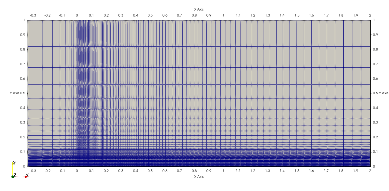
メッシュサイズの分割数は以下の部分で調整することができます。
|
1 2 3 4 5 6 7 8 9 10 11 12 13 14 |
blocks ( hex (0 1 5 4 3 2 6 7) (100 1 50) simpleGrading (20 1 5) hex (11 0 4 10 9 3 7 8) (10 1 50) simpleGrading (0.05 1 5) hex (9 3 7 8 14 13 16 15) (10 1 18) simpleGrading (0.05 1 40) hex (3 2 6 7 13 12 17 16) (100 1 18) simpleGrading (20 1 40) /* hex (0 1 5 4 3 2 6 7) (100 1 225) simpleGrading (20 1 500) hex (11 0 4 10 9 3 7 8) (20 1 225) simpleGrading (0.05 1 500) hex (9 3 7 8 14 13 16 15) (20 1 10) simpleGrading (0.05 1 20) hex (3 2 6 7 13 12 17 16) (100 1 10) simpleGrading (20 1 20) */ ); |
メッシュサイズは$y^+$に関わってくるため重要な要素だということを覚えておきましょう。
解析設定
物性値の設定
物性値はconstant/transportPropertiesで設定を行います。
非圧縮流れにおいての物性値は動粘性係数$\nu\text{m}^2/\text{s}$だけです。
|
1 2 3 |
transportModel Newtonian; nu 2e-07; |
流入速度$U=1.0\text{m}/\text{s}$ですので、レイノルズ数は$Re=\frac{UL}{\nu}=\frac{1.0\times 2}{2\times 10^{-7}}=10^7$となります。
乱流モデル
乱流モデルは$k$-$\omega$SSTを使用します。
$k$-$\omega$SSTモデル(Shear Stress Transportモデル)は、乱流モデルの中でも広く利用されているモデルの一つで、以下の特長を持ちます。
- $k$-$\omega$モデルと$k$-$\varepsilon$モデルのハイブリッド
- 壁近傍では$k$-$\omega$モデルを使用し、壁面に近い部分での精度を高めます。
- 壁面から離れた部分では$k$-$\varepsilon$モデルを使用し、自由流の挙動を適切に予測します。
- せん断応力輸送(SST)モデル
- 境界層剥離などのせん断応力が重要な現象をより正確に捉えるため、せん断応力を考慮する形に改良されています。
- 境界層内の分離挙動を精度よく予測する能力があります。
次回の記事では$k$-$\varepsilon$と$k$-$\omega$SSTとの結果の違いも見ていきたいと思います。
離散化スキーム
system/fvSchemesで離散化のスキームの設定を行います。
特に粘性項のない場合の移流方程式などでは、対流項のスキームによってかなり結果が変わることもあります。
今回は粘性項も圧力項もあるのでスキームの違いによる大きな変化はないかもしれません。
system/fvSchemes
|
1 2 3 4 5 6 7 8 9 10 11 12 13 14 15 16 17 18 19 20 21 22 23 24 25 26 27 28 29 30 31 32 33 34 35 36 37 38 39 40 41 42 |
ddtSchemes { default steadyState; } gradSchemes { // default Gauss linear; default cellLimited Gauss linear 1; } divSchemes { default none; div(phi,U) bounded Gauss linearUpwind grad(U); div(phi,k) bounded Gauss limitedLinear 1; div(phi,epsilon) bounded Gauss limitedLinear 1; div(phi,omega) bounded Gauss limitedLinear 1; div(phi,v2) bounded Gauss limitedLinear 1; div((nuEff*dev2(T(grad(U))))) Gauss linear; div(nonlinearStress) Gauss linear; } laplacianSchemes { default Gauss linear corrected; } interpolationSchemes { default linear; } snGradSchemes { default corrected; } wallDist { method meshWave; } |
興味があれば色々と変更して遊んでみてください。
代数ソルバ
system/fvSolutionで行列解法の設定を行います。
system/fvSolution
|
1 2 3 4 5 6 7 8 9 10 11 12 13 14 15 16 17 18 19 20 21 22 23 24 25 26 27 28 29 30 31 32 33 34 35 36 37 38 39 40 41 42 43 44 45 46 47 48 |
solvers { p { // solver GAMG; // tolerance 1e-06; // relTol 0.1; // smoother GaussSeidel; solver PCG; preconditioner DIC; tolerance 1e-6; relTol 0.01; } "(U|k|epsilon|omega|f|v2)" { // solver smoothSolver; // smoother symGaussSeidel; // tolerance 1e-05; // relTol 0.1; solver PBiCGStab; preconditioner DILU; tolerance 1e-8; relTol 0; } } SIMPLE { nNonOrthogonalCorrectors 0; consistent yes; residualControl { p 1e-6; U 1e-6; "(k|epsilon|omega|f|v2)" 1e-6; } } relaxationFactors { equations { U 0.7; // 0.9 is more stable but 0.95 more convergent ".*" 0.7; // 0.9 is more stable but 0.95 more convergent } } |
計算が発散する場合はrelaxationFactorsなどの数値を小さくしてどうなるか様子を見てください。
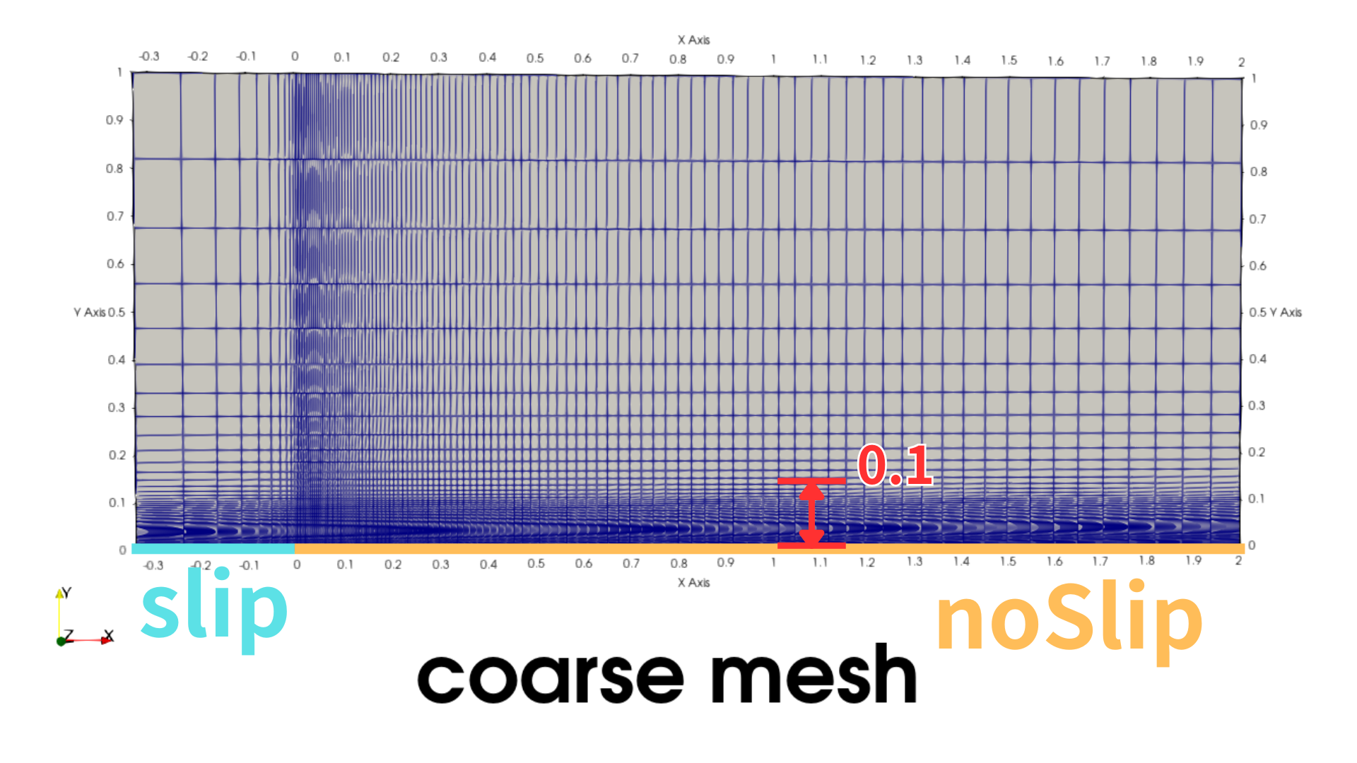
境界条件
それぞれの境界面の名前は以下のようになっており、各面に対して適切な設定する必要があります。
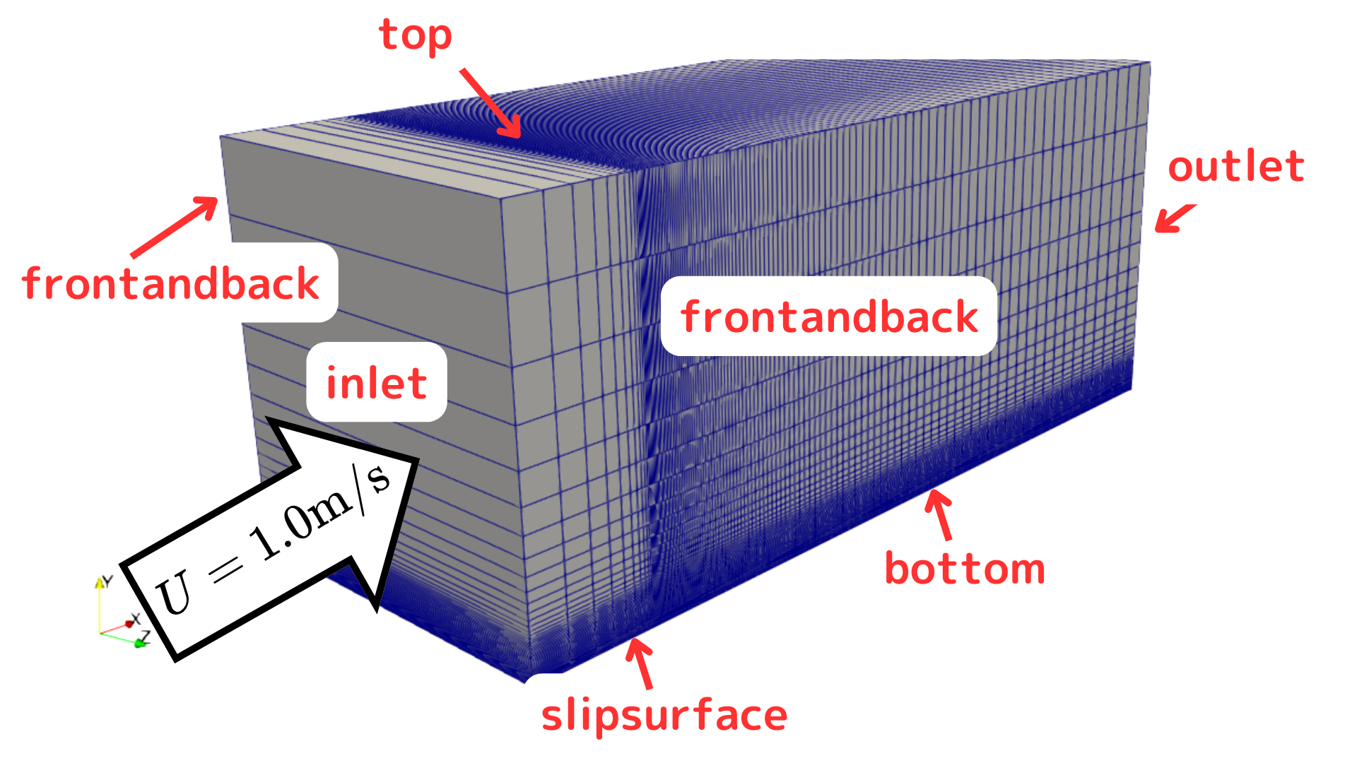
$k$-$\omega$SSTに必要な境界条件として以下となります。
U: 流速ベクトル場p: 圧力場k: 乱流運動エネルギーomega: 比乱流散逸率nut: 乱流粘性係数
U: 流速ベクトル場
|
1 2 3 4 5 6 7 8 9 10 11 12 13 14 15 16 17 18 19 20 21 22 23 24 25 26 27 28 29 30 31 32 33 34 35 36 37 38 39 |
dimensions [0 1 -1 0 0 0 0]; internalField uniform (1 0 0); boundaryField { inlet { type fixedValue; value uniform (1 0 0); } outlet { type zeroGradient; } top { type zeroGradient; } bottom { type fixedValue; value uniform (0 0 0); } slipsurface { //type zeroGradient; type slip; } frontandback { type empty; } } |
p: 圧力場
|
1 2 3 4 5 6 7 8 9 10 11 12 13 14 15 16 17 18 19 20 21 22 23 24 25 26 27 28 29 30 31 32 33 34 35 36 |
dimensions [0 2 -2 0 0 0 0]; internalField uniform 0; boundaryField { inlet { type zeroGradient; } outlet { type fixedValue; value uniform 0; } top { type zeroGradient; } bottom { type zeroGradient; } slipsurface { //type zeroGradient; type slip; } frontandback { type empty; } } |
以下、壁関数の設定を含む乱流モデルの変数の設定です。
壁関数については、こちらにわかりやすくまとめられています。
k: 乱流運動エネルギー
|
1 2 3 4 5 6 7 8 9 10 11 12 13 14 15 16 17 18 19 20 21 22 23 24 25 26 27 28 29 30 31 32 33 34 35 36 37 38 39 40 41 42 43 44 45 46 |
dimensions [0 2 -2 0 0 0 0]; //internalField uniform 1e-09; internalField uniform 0.00015; boundaryField { inlet { type fixedValue; value $internalField; } top { type zeroGradient; } outlet { type zeroGradient; } slipsurface { //type zeroGradient; type slip; } bottom { //type fixedValue; //value $internalField; //value uniform 1e-12; //To use wall functions type kqRWallFunction; //value uniform 1e-09; value $internalField; } frontandback { type empty; } } |
omega: 比乱流散逸率
|
1 2 3 4 5 6 7 8 9 10 11 12 13 14 15 16 17 18 19 20 21 22 23 24 25 26 27 28 29 30 31 32 33 34 35 36 37 38 39 40 41 42 43 |
dimensions [0 0 -1 0 0 0 0]; //internalField uniform 5; internalField uniform 750; boundaryField { inlet { type fixedValue; value $internalField; } top { type zeroGradient; } outlet { type zeroGradient; } slipsurface { //type zeroGradient; type slip; } bottom { //type fixedValue; //value uniform 4000000; //value uniform 1e-12; //value $internalField; //Must be on - To enable wall function - Both values give right resutls type omegaWallFunction; value $internalField; //value uniform 4000000; } frontandback { type empty; } } |
nut: 乱流粘性係数
|
1 2 3 4 5 6 7 8 9 10 11 12 13 14 15 16 17 18 19 20 21 22 23 24 25 26 27 28 29 30 31 32 33 34 35 36 37 38 39 40 41 42 43 |
dimensions [0 2 -1 0 0 0 0]; //1 to 10 times laminar vis internalField uniform 2e-07; boundaryField { inlet { type calculated; value uniform 0; } top { type calculated; value uniform 0; } outlet { type calculated; value uniform 0; } slipsurface { //type zeroGradient; type slip; } bottom { //type fixedValue; //value uniform 0; // type nutUSpaldingWallFunction; // value uniform 0; type nutkWallFunction; value uniform 0; } frontandback { type empty; } } |
計算制御設定
system/controlDictで計算に関する設定を行います。
また、functionsで出力設定なども行います。
|
1 2 3 4 5 6 7 8 9 10 11 12 13 14 15 16 17 18 19 20 21 22 23 24 25 26 27 28 29 30 31 32 33 34 35 36 37 38 39 40 41 42 43 44 45 46 47 48 49 50 51 52 53 54 55 56 57 58 59 60 61 62 63 64 65 66 67 |
application simpleFoam; startFrom startTime; startTime 0; stopAt endTime; endTime 2000; deltaT 1; writeControl timeStep; writeInterval 100; purgeWrite 3; writeFormat ascii; writePrecision 6; writeCompression off; timeFormat general; timePrecision 6; runTimeModifiable true; functions { #includeFunc yPlus continuityError1 { type continuityError; libs ( fieldFunctionObjects ); // Mandatory entries (unmodifiable)// Optional entries (runtime modifiable) phi phi; // Optional (inherited) entries writePrecision 8; writeToFile yes; useUserTime yes; region region0; enabled yes; log yes; timeStart 0; timeEnd 6000; executeControl timeStep; executeInterval 1; writeControl timeStep; writeInterval 50; } residuals { type solverInfo; libs ( "libutilityFunctionObjects.so" ); fields ( ".*" ); } } |
- ypuls:$y^+$
- continuityError:連続式の誤差
- residuals:残差
これらの設定を行います。
また、system/sampleDictで物理量の出力設定も行います。
system/sampleDict
|
1 2 3 4 5 6 7 8 9 10 11 12 13 14 15 16 17 18 19 20 21 22 23 24 25 26 27 28 29 |
sampleDict { type sets; libs (sampling); setFormat raw; interpolationScheme cellPoint;//cell; fields (U k nut omega wallShearStress); writeControl writeTime; sets ( profile0 // inlet patch face centres { type face; axis distance;//y; start (1.90334 0 0); end (1.90334 0.1 0); //y 0.1 nPoints 1000; } profile1 // inlet patch face centres { type uniform;//face; axis distance;//y; start (-0.1 0 0); end (2 0 0); nPoints 1000; } ); } |
profile0で$x=1.90334$の位置で、$y$方向に$0~0.1$の物理量をサンプルとして出力する設定にしています。
profile1はおまけで設定します。
以上で解析設定が終わりました。
計算の実行
では、計算の実行を行います。
ここでは、
- 計算実行
- 各ステップの物理量の出力
- ある座標軸での物理量の出力
を行うためにAllrunスクリプトにコマンドをまとめておきます。
|
1 2 3 4 5 6 7 8 9 10 11 12 13 14 15 16 17 18 19 |
#!/bin/bash # スクリプトのエラーを早期に検出するための設定 set -e # コマンドが失敗した場合にスクリプトを停止する set -o pipefail # パイプライン内のいずれかのコマンドが失敗した場合に停止する # simpleFoamの実行 echo "Running simpleFoam..." simpleFoam # wallShearStressの計算 echo "Calculating wallShearStress..." simpleFoam -postProcess -func wallShearStress -noZero -noFunctionObjects # sampleDictによるデータ抽出 echo "Sampling data with sampleDict..." postProcess -func sampleDict -latestTime echo "All processes completed successfully!" |
では、Allrunスクリプトを実行します。
|
1 |
./Allrun |
計算ログが出力されて終了します。
|
1 2 3 4 5 6 7 8 9 10 11 12 13 14 15 16 17 18 19 20 21 22 23 24 25 26 27 28 29 30 31 32 33 34 35 |
ExecutionTime = 28.54 s ClockTime = 47 s Time = 2000 DILUPBiCGStab: Solving for Ux, Initial residual = 4.86091e-05, Final residual = 5.86885e-09, No Iterations 1 DILUPBiCGStab: Solving for Uy, Initial residual = 0.000513335, Final residual = 5.046e-09, No Iterations 1 DICPCG: Solving for p, Initial residual = 0.00209287, Final residual = 1.86888e-05, No Iterations 19 time step continuity errors : sum local = 2.1418e-07, global = -4.04014e-08, cumulative = -3.96229e-07 DILUPBiCGStab: Solving for omega, Initial residual = 2.25983e-05, Final residual = 4.59429e-09, No Iterations 1 DILUPBiCGStab: Solving for k, Initial residual = 2.17709e-05, Final residual = 6.48659e-10, No Iterations 2 ExecutionTime = 28.58 s ClockTime = 48 s yPlus yPlus write: writing field yPlus patch bottom y+ : min = 11.9464, max = 91.0129, average = 71.4975 continuityError continuityError1 write: local = 2.1418e-07 global = -4.04014e-08 cumulative = -3.44755e-08 End ...(省略)... Time = 2000 Reading fields: volScalarField: k nut omega volVectorField: U wallShearStress Executing functionObjects End All processes completed successfully! |
結果のグラフ化
まずは$y^+$を確認してみましょう。
$y+$の確認
$y^+$を確認するPythonプログラムを載せておきます。
|
1 2 3 4 5 6 7 8 9 10 11 12 13 14 15 16 17 18 19 20 21 22 23 24 25 26 27 28 29 30 31 32 |
import pandas as pd import matplotlib.pyplot as plt def graph_layout(): plt.grid() plt.legend(loc='best',bbox_to_anchor=(1, 1)) plt.yscale('log') plt.xlabel('time', fontsize=16) plt.ylabel('df_yPlus', fontsize=16) plt.savefig("yPlus.png") def df_yPlus_func(dir_): df_yPlus = pd.read_table(f'./postProcessing/yPlus/{dir_}/yPlus.dat',skiprows=1) df_yPlus = pd.DataFrame(df_yPlus) return df_yPlus def df_concat(dir_List): df = pd.DataFrame() for dir_ in dir_List: try: df_ = df_yPlus_func(dir_) df = pd.concat([df, df_]) except Exception: print("Empty") return df df_yPlus = pd.DataFrame() dir_List = os.listdir('./postProcessing/yPlus') df_yPlus = df_concat(dir_List) time = df_yPlus.columns[0] df_yPlus[df_yPlus[time]==df_yPlus[time].max()] |
|
1 2 |
# Time patch min max average 19 2000 bottom 11.94642 91.01288 71.49747 |
壁面bottomの$y^+$は平均で71.49747となっています。
高レイノルズ型の乱流モデル$k$-$\varepsilon$であれば$y^+ \geq 30$は必要なのでOKそうですね。今回は、$k$-$\omega$SSTモデルなので、あまり厳しい$y^+$の縛りはないですが。
$y^+$-$u^+$の確認
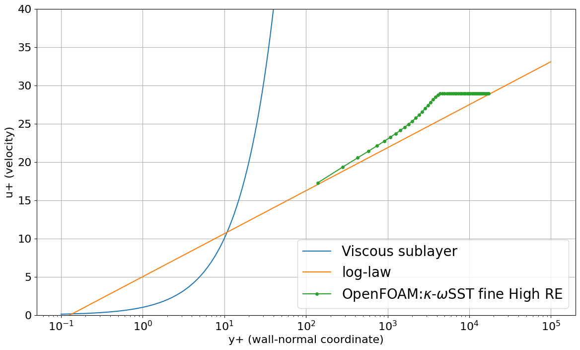
壁からの距離$y$を横軸に、壁と水平方向($x$方向)の流速$u$を縦軸にとった以下のグラフとOpenFOAMの結果とを比較してみましょう。
※グラフは復習のため再度載せておきます。
- $y^{+}=\frac{u_{\tau}y}{\nu}$
- $u^{+}=\frac{u}{u^{\tau}}$
※$u_{\tau}=\sqrt{\frac{\tau_{w}}{\rho}}$:摩擦速度
※$\tau_{w}=\mu\frac{\partial u}{\partial y}$:壁面のせん断力
※$\kappa=0.41, C = 5.0$
では、OpenFOAMの結果をPythonで可視化し、上記理論式との比較を行います。
|
1 2 3 4 5 6 7 8 9 10 11 12 13 14 15 16 17 18 19 20 21 22 23 24 25 26 27 28 29 30 31 32 33 34 35 36 37 38 39 40 41 42 43 44 45 46 47 48 49 50 51 52 53 54 55 56 57 58 59 60 61 |
import numpy as np import matplotlib.pyplot as plt from scipy import interpolate kwhre_0 = np.loadtxt("postProcessing/sampleDict/2000/profile0_k_nut_omega_U_wallShearStress.xy",skiprows=0) #kwhre_1 = np.loadtxt("postProcessing/sampleDict/2000/profile1_U_wallShearStress.xy",skiprows=0) #Compute therorical profiles yp=np.linspace(0.1,100000,1000000) #Laminar up_vis=yp #Low-law up_log=(1.0/0.41)*np.log(yp)+5.0 #Where to sample xloc=1.90334 #Input values U = 1 nu = 2.0e-07 rho = 1.0 #fint1=interpolate.interp1d(kwhre_1[:,0],kwhre_1[:,4],kind='linear') #KW HIGH RE ws = np.sqrt(kwhre_0[:,7]**2 + kwhre_0[:,8]**2 + kwhre_0[:,9]**2) um = np.sqrt(kwhre_0[:,4]**2 + kwhre_0[:,5]**2 + kwhre_0[:,6]**2) #wsm=0.0012264945506493506 wsm=np.abs(kwhre_0[0,7]) #np.abs(fint1(xloc)) print(wsm) print(np.abs(kwhre_0[0,7])) utau=np.sqrt(wsm/rho) ypn=utau*kwhre_0[:,0]/nu upn=um/utau #Plot profiles # Plot profiles plt.figure(figsize=(14, 8)) # Correlations plt.plot(yp, up_vis, label='Viscous sublayer') plt.plot(yp, up_log, label='log-law') # OpenFOAM plt.plot(ypn[1:], upn[1:], '-o', ms=4, label='$\kappa$-$\omega$ High RE') plt.xscale('log') plt.ylim(0, 40) # ラベルとフォントサイズの設定 plt.xlabel('y+ (wall-normal coordinate)', fontsize=16) # 横軸ラベル plt.ylabel('u+ (velocity)', fontsize=16) # 縦軸ラベル # 目盛りのフォントサイズを変更 plt.tick_params(axis='both', which='major', labelsize=16) plt.tick_params(axis='both', which='minor', labelsize=12) plt.grid() plt.legend(loc=2, fontsize=20) |
計算方法は、まずws = np.sqrt(kwhre_0[:,7]**2 + kwhre_0[:,8]**2 + kwhre_0[:,9]**2)とwsm=np.abs(kwhre_0[0,7]) より壁面の摩擦せん断力$\tau_w$を計算します。
そして、utau=np.sqrt(wsm/rho)で摩擦速度を$u_{\tau}=\sqrt{\frac{\tau_{w}}{\rho}}$を、ypn=utau*kwhre_0[:,0]/nuで$y^{+}=\frac{u_{\tau}y}{\nu}$を、upn=um/utauで$u^{+}=\frac{u}{u_{\tau}}$を計算しています。
横軸$y^{+}$、縦軸u^{+}$にしたのが下のグラフです。
- Viscous sublayar:$u^{+}=y^{+}$
- log-law:$u^{+}=\frac{1}{\kappa}\log_{10}y^{+}+C$
※$\kappa=0.41, C = 5.0$
 乱流の対数域の線に乗っているかどうか微妙なところですが、概ね理論通りでしょう。
まとめ
今回は、平板流れのモデル作成を通じて、乱流モデルと壁関数の設定方法について解説しました。また、$y^+$と$u^+$の関係を確認し、理論と一致しているかを可視化して検証するプロセスもご紹介しました。
次回は、さらに一歩踏み込んで、他の乱流モデル(例:$k$-$\varepsilon$モデルや低レイノルズ数型モデル)、別の壁関数の適用、さらには壁関数を使用しない場合の設定など、多様な条件下で結果がどのように異なるのかを比較・検証していきたいと思います。
計算力学技術者のための問題アプリ
計算力学技術者熱流体2級、1級対策アプリをリリースしました。
- 下記をクリックしてホームページでダウンロードできます。
- LINE公式に登録すると無料で問題の一部を閲覧できます。
※LINEの仕様で数式がずれていますが、アプリでは問題ありません。
- 計算力学技術者の熱流体2級問題アプリ作成
リリース後も試行錯誤をしながら改善に努め日々アップデートしています。
備忘録として作成の過程を綴っています。
お勧めの参考書
乱流モデルの数式の展開が非常に丁寧なのはこちらの参考書です。
今まで読んだ本の中で途中式もしっかり書いてあって一番丁寧でした。
乱流モデルの話だけでなく、混相流(気液、固液)や粒子法、浅水方程式の話も乗っているので重宝しています。
乱流モデルはこちらもお勧めです。
前半は数値シミュレーションの離散化の話で、後半に乱流モデルの話が出てきます。
乱流モデルのざっくりした解説と流体全般の基礎知識にはこちらがちょうど良いでしょう。