こんにちは(@t_kun_kamakiri)
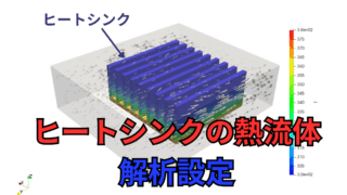
OpenFOAMの熱流体固体連成によるヒートシンクの熱流体解析の設定方法を解説します。
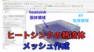
前回メッシュ作成まで行いましたので、メッシュ作成編を見たい方はこちらをどうぞ。

使用するソルバはchtMultiRegionSimpleFoamで熱流体と固体を連成させた定常解析用のソルバになります。
OpenFOAMv2412のバージョンにおいて現在は、浮力を考慮した熱流体解析ソルバは以下のものがあります。
| ソルバ名 | 定常 / 非定常 | 主な特徴 | 主な用途・備考 |
|---|---|---|---|
chtMultiRegionSimpleFoam | 定常 | 多領域の熱流体連成(非圧縮性) | 構造物と流体の熱連成、定常問題向け |
chtMultiRegionFoam | 非定常 | 多領域・非圧縮性の時間依存連成解析 | 熱伝導と流体連成の過渡解析 |
chtMultiRegionTwoPhaseEulerFoam | 非定常 | 多領域 + 二相流(Euler-Euler) + 熱連成 | 液体/気体の二相流+固体との熱連成に対応 |
buoyantSimpleFoam | 定常 | 単領域の自然対流・熱伝導 | 密度差による自然対流、定常解析向け |
buoyantPimpleFoam | 非定常 | 上記の非定常版 | 過渡的な自然対流解析 |
buoyantBoussinesqSimpleFoam | 定常 | Boussinesq近似(小温度差) | 温度変化が小さい自然対流 |
buoyantBoussinesqPimpleFoam | 非定常 | 上記の時間依存版 | 過渡的自然対流、簡略化モデル |
この中のchtMultiRegion系は流体(液体、気体)・固体の複数領域の熱流体解析を行うために設計されています。
ただ、テキストベースで解析設定しようとすると、めちゃくちゃ大変です。
以下にOpenFOAMが用意しているチュートリアルを解説した記事がありますので、一度読んでみると良いでしょう。
以前にsappyHexMeshでヒートシンクの固体・流体連成の解析を紹介しました。
今回は違った方法でモデル作成を行いヒートシンクの解析まで行います。
領域分割やメッシュ作成はSALOMEを使用します。
SALOMEを使ったマルチリージョン用メッシュからOpenFOAMでの流体解析の手順を紹介します。
OpenFOAM v2412(WSL Ubuntu 22.04)
SALOME 9.15.0
OpenFOAM用の設定ファイルの準備
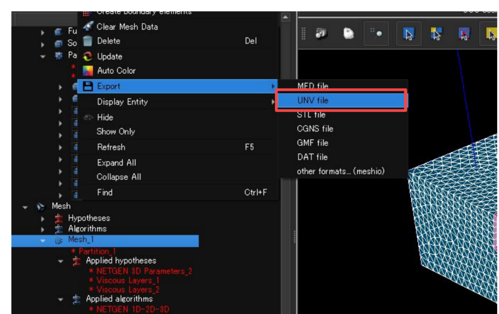
SALOMEで問題なくメッシュ作成と境界の設定が終わったらOpenFOAMの形式に変換します。
以下のようにunvファイルとして出力します。
出力したunvファイルをOpenFOAM形式に変換するにはダミーのケースファイルが必要です。適当なチュートリアルからコピーしてきます。
今回は固体・熱流体の定常解析で計算するのでchtMultiRegionSimpleFoamからコピーしてきます。
|
1 |
cp -r /home/kamakiri/repo/openfoam/tutorials/heatTransfer/chtMultiRegionSimpleFoam/cpuCabinet/ |
$FOAM_TUTORIALS = /home/kamakiri/repo/openfoam/tutorials
salomeで作成したunvファイルをケースファイルに保存します。
|
1 |
cp -r model/Mesh_1.unv . |
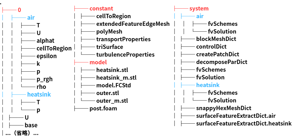
今フォルダ構成を確認してくと以下のようになっています。
|
1 2 3 4 5 6 7 8 9 10 11 12 13 14 15 16 17 18 19 20 21 22 23 24 25 26 27 28 29 30 31 32 33 34 35 |
. ├── 0.orig │ ├── domain0 │ ├── v_CPU │ └── v_fins ├── Allclean ├── Allrun ├── Allrun.pre ├── Mesh_1.unv ├── constant │ ├── domain0 │ ├── g │ ├── regionProperties │ ├── v_CPU │ └── v_fins ├── model │ ├── Mesh_1.unv │ ├── Study1.hdf │ ├── heatsinkl.step │ └── model.FCStd └── system ├── blockMeshDict ├── controlDict ├── createBafflesDict ├── decomposeParDict ├── domain0 ├── fvSchemes ├── fvSolution ├── meshQualityDict ├── probes ├── snappyHexMeshDict ├── surfaceFeatureExtractDict ├── topoSetDict.f1 ├── v_CPU └── v_fins |
0.origをコピーします。
|
1 |
cp -r 0.orig 0 |
すでに0フォルダにあるフォルダをひとまずoldフォルダに避難させます。
|
1 2 3 |
mkdir -p 0/old && mv 0/{domain0,v_CPU,v_fins} 0/old mkdir -p constant/old && mv constant/{domain0,v_CPU,v_fins} constant/old mkdir -p system/old && mv system/{domain0,v_CPU,v_fins} system/old |
ここからがマルチリージョンソルバの手順のコツですが、以下のように0フォルダに計算する物理量のファイルを用意します。
今回はk-ωSSTの乱流モデルで計算したいので必要なのは、U,T,p_rgh,p,k,omega,nut,alphatになります。
|
1 2 3 4 5 6 7 8 9 10 11 12 13 |
0 ├── T ├── U ├── alphat ├── cellToRegion ├── epsilon ├── k ├── nut ├── old ├── omega ├── p ├── p_rgh └── rho |
中身はすべて以下としておきます。
例としてUの中身を示しています。物理量によってdimensionsが異なるので注意してください。適当なチュートリアルから各物理量をコピーしてきて、以下のように編集しておくとよいでしょう。
|
1 2 3 4 5 6 7 8 9 10 11 12 13 14 15 16 17 18 19 20 21 22 23 |
FoamFile { version 2.0; format ascii; class volVectorField; object U; } // * * * * * * * * * * * * * * * * * * * * * * * * * * * * * * * * * * * * * // dimensions [0 1 -1 0 0 0 0]; internalField uniform (0.01 0 0); boundaryField { #includeEtc "caseDicts/setConstraintTypes" ".*" { type calculated; value $internalField; } } |
こうしておくと非常に便利です。
このあと0, constant, systemフォルダに各領域のフォルダを作っていく必要があるのですが、これを手動で行うとめちゃくちゃ面倒になります。
ぜひ、以下の方法を覚えておいてください。
OpenFOAMの形式に変換
ここからSALOMEで作成したメッシュ情報をOpenFOAMに変換します。
以下のコマンドでOpenFOAMの形式に変換します。
|
1 |
ideasUnvToFoam Mesh_1.unv |
エラーがなければconstant/polyMeshフォルダが作成されOpenFOAMのメッシュ情報が作られています。
※今回は必要ありませんが、salomeではmm単位のつもりで作成しましたが、実は数値しか意味がなく、OpenFOAMでの計算がm単位なので、必要に応じて以下のコマンドでスケールを1/1000倍にします。
|
1 |
transformPoints -scale '(0.001 0.001 0.001)' |
再度、モデルの大きさを確認します。
まだメッシュを変換しただけで領域ごとにメッシュが分かれているわけではありません。以下のコマンドで領域を分割します。
|
1 |
splitMeshRegions -cellZones -overwrite |
領域分割によりフォルダ構成は以下となっています。
splitMeshRegionsコマンドにより、0, constant. system内に領域ごとの設定ファイルが作成されますconstant/air(heatsink), system/air(heatsink)のフォルダは元々作成していましたが、0/air(heatsink)はフォルダが生成されたと思います。
気体領域と固体領域で共通している面は、heatsink_to_airやair_to_heatsinkの名前が付けられます。
境界条件の設定
splitMeshRegionsコマンドにより境界条件の設定ファイルの中身も変わっています。
例として流速の0フォルダを示します。
0/air/U
|
1 2 3 4 5 6 7 8 9 10 11 12 13 14 15 16 17 18 19 20 21 22 23 24 25 26 27 28 29 30 31 32 33 34 35 36 37 38 39 40 41 42 |
dimensions [0 1 -1 0 0 0 0]; internalField uniform (0.01 0 0); boundaryField { YMin { type calculated; value uniform (0.01 0 0); } ZMax { type calculated; value uniform (0.01 0 0); } YMax { type calculated; value uniform (0.01 0 0); } XMin { type calculated; value uniform (0.01 0 0); } ZMin { type calculated; value uniform (0.01 0 0); } XMax { type calculated; value uniform (0.01 0 0); } air_to_heatsink { type calculated; value uniform (0 0 0); } } |
このように自動的にair領域の境界条件が作成されています。
ここで注意として、流体領域と固体領域で必要になるファイルが異なります。
- 流体領域:0, T, p_rgh, p
- 固体領域:T, p
k-ωSST乱流モデルを使用するのであれば、流体領域にさらにk, omega, nut, alphatが必要になります。
さてここから境界条件を手動で競ってしていきたいところですが、まだ手動で行うには少々面倒なのでchangeDictionaryDictを使用します。
以下では境界条件の設定と同時にconstant/<region>/polyMesh/boundaryの境界のタイプも変更しています。
system/air/changeDictionaryDict
|
1 2 3 4 5 6 7 8 9 10 11 12 13 14 15 16 17 18 19 20 21 22 23 24 25 26 27 28 29 30 31 32 33 34 35 36 37 38 39 40 41 42 43 44 45 46 47 48 49 50 51 52 53 54 55 56 57 58 59 60 61 62 63 64 65 66 67 68 69 70 71 72 73 74 75 76 77 78 79 80 81 82 83 84 85 86 87 88 89 90 91 92 93 94 95 96 97 98 99 100 101 102 103 104 105 106 107 108 109 110 111 112 113 114 115 116 117 118 119 120 121 122 123 124 125 126 127 128 129 130 131 132 133 134 135 136 137 138 139 140 141 142 143 144 145 146 147 148 149 150 151 152 153 154 155 156 157 158 159 160 161 162 163 164 165 166 167 168 169 170 171 172 173 174 175 176 177 178 179 180 181 182 183 184 185 186 187 188 189 190 191 192 193 194 195 196 197 198 199 200 201 202 203 204 205 206 207 208 209 210 211 212 213 214 215 216 217 218 219 220 221 222 223 224 225 226 227 228 229 230 231 232 233 234 235 236 237 238 239 240 241 242 243 244 245 246 247 248 249 250 251 252 253 254 255 256 257 258 259 260 261 262 263 264 265 266 267 268 269 270 271 272 273 274 275 276 |
boundary { ".*" { type wall; } ".*_to_.*" { type mappedWall;; } YMin { type patch; } YMax { type patch; } } k { internalField uniform 0.00375; boundaryField { ".*" { type kqRWallFunction; value $internalField; } YMin { type inletOutlet; inletValue uniform 0.00375; value uniform 0.00375; } YMax { type turbulentIntensityKineticEnergyInlet; value $internalField; intensity 0.03; } } } omega { internalField uniform 5.6;////I=0.05,k=3/2(IU)^2, omega=k^0.5/(Cnu^0.25*L),L=20 boundaryField { ".*" { type omegaWallFunction; value $internalField; } YMin { type inletOutlet; inletValue uniform 0.67082; value uniform 6.7082e-05; } YMax { type turbulentMixingLengthFrequencyInlet; mixingLength 0.01; value uniform 0.67082; } } } nut { internalField uniform 6000; boundaryField { ".*" { type nutkWallFunction; value uniform 0; } YMin { type calculated; value uniform 0; } YMax { type calculated; value uniform 0; } } } U { internalField uniform ( 0 -0.5 0 ); boundaryField { ".*" { type fixedValue; value uniform (0 0 0); } YMin { type pressureInletOutletVelocity; value $internalField; } YMax { type fixedValue; value $internalField; } } } T { internalField uniform 293.15; boundaryField { ".*" { type fixedValue; value uniform 293.15; } YMin { type fixedValue; value uniform 293.15; } YMax { type zeroGradient; } ".*_to_.*" { type compressible::turbulentTemperatureRadCoupledMixed; value uniform 293.15; Tnbr T; kappaMethod fluidThermo; qrNbr none; qr none;//qr; thermalInertia true; kappa none; } } } p_rgh { internalField uniform 100000; boundaryField { ".*" { type fixedFluxPressure; value uniform 100000; } YMin { type totalPressure; value uniform 100000; p0 uniform 100000; } YMax { type fixedFluxPressure; value uniform 100000; } } } p { internalField uniform 100000; boundaryField { ".*" { type calculated; value uniform 100000; } } } alphat { internalField uniform 0; boundaryField { ".*" { type compressible::alphatWallFunction; Prt 0.85; value uniform 0; } YMin { type calculated; value uniform 0; } YMax { type calculated; value uniform 0; } } } G { internalField uniform 0; boundaryField { ".*" { type MarshakRadiation; value uniform 0; } } } qr { internalField uniform 0; boundaryField { ".*" { type calculated; value uniform 0; } } } IDefault { internalField uniform 0; boundaryField { ".*" { type greyDiffusiveRadiation; value uniform 0; } } } |
G, qr, IDefaultなどはふく射の設定時に使うものなのですが、一応書いておきます(ふく射計算する際には使用する場合もあります)
system/heatsink/changeDictionaryDict
|
1 2 3 4 5 6 7 8 9 10 11 12 13 14 15 16 17 18 19 20 21 22 23 24 25 26 27 28 29 30 31 32 33 34 35 36 37 38 39 40 41 42 43 44 45 46 47 48 49 50 51 52 53 54 55 56 57 58 |
boundary { ".*" { type wall; } ".*_to_.*" { type mappedWall;; } YMin { type patch; } YMax { type patch; } } T { internalField uniform 293.15; // 初期固体温度 boundaryField { // すべての固体外表面は固定温度(必要に応じて zeroGradient に変更可) ".*" { type fixedValue; value uniform 293.15; } heatSource { type externalWallHeatFluxTemperature; value $internalField; kappaMethod fluidThermo; mode power; Ta $internalField; Q uniform 2000; kappaName none; } // 流体-固体連成面 ".*_to_.*" { type compressible::turbulentTemperatureRadCoupledMixed; Tnbr T; kappaMethod solidThermo; qrNbr none; qr none; kappa none; thermalInertia true; value uniform 293.15; } } } |
設定を終わった後に領域を指定する必要があるので、以下の設定ファイルを変更します。
constant/regionProperties
|
1 2 3 4 5 |
regions ( solid ( heatsink ) fluid ( air ) ); |
ここから以下のコマンドで領域ごとに境界条件を指定します。
|
1 |
for region in $(foamListRegions); do changeDictionary -region "$region"; done |
このコマンドは;で区切ることで次のコマンドを打っていることになるので、スクリプトとして書くならばインデントをきれいにして以下のように書きます。
|
1 2 3 4 |
for region in $(foamListRegions) do changeDictionary -region "$region" done |
これにより協会条件が各領域の各面で設定されたのではないかと思います。
物性値の設定
ここから各領域の物性値を設定します。
物性値はconstantフォルダにあります。
|
1 2 |
cp -r constant/old/domain0/thermophysicalProperties constant/air/ cp -r constant/old/v_CPU/thermophysicalProperties constant/heatsink/ |
まずは流体領域の空気の物性値を指定します。
constant/air/thermophysicalProperties
|
1 2 3 4 5 6 7 8 9 10 11 12 13 14 15 16 17 18 19 20 21 22 23 24 25 26 27 28 29 30 31 |
thermoType { type heRhoThermo; mixture pureMixture; transport const; thermo hConst; equationOfState perfectGas; specie specie; energy sensibleEnthalpy; } mixture { specie { nMoles 1; molWeight 28.966; } thermodynamics { Cp 1006.43; Hf 0; } transport { mu 1.846e-05; Pr 0.706414; } } |
固体領域はアルミニウム(Al)の固体物性値とします。
constant/heatsink/thermophysicalProperties
|
1 2 3 4 5 6 7 8 9 10 11 12 13 14 15 16 17 18 19 20 21 22 23 24 25 26 27 28 29 30 31 32 33 34 35 36 |
thermoType { type heSolidThermo; mixture pureMixture; transport constIso; thermo hConst; equationOfState rhoConst; specie specie; energy sensibleEnthalpy; } mixture { specie { nMoles 1; molWeight 26.98; } thermodynamics { Hf 0; Sf 0; Cp 871; } transport { kappa 202.4; } equationOfState { rho 2719; } } |
また流体と固体では状態方程式を扱うモデルが違うことに注意してください。
- 流体領域:equationOfState perfectGas;理想気体の状態方程式
- 固体領域:equationOfState rhoConst;密度一定
乱流モデルの設定
乱流モデルもチュートリアルの設定からコピーしてきます。
|
1 |
cp -r constant/old/domain0/turbulenceProperties constant/air/ |
乱流モデルの設定はk-ωSSTにしたいので以下のように変更します。
|
1 2 3 4 5 6 7 8 |
simulationType RAS; RAS { RASModel kOmegaSST;//realizableKE; turbulence on; printCoeffs on; } |
重力の設定
重力はz方向の負の方向に指定します。
これの向きを間違えると浮力流れの向きがおかしくなります。
constant/g
|
1 2 3 |
dimensions [0 1 -2 0 0 0 0]; value (0 0 -9.81); |
離散化・代数ソルバ
こちらもチュートリアルからコピーしてきます。
|
1 2 |
cp -r system/old/domain0/{fvSchemes,fvSolution} system/air/ cp -r system/old/v_CPU/{fvSchemes,fvSolution} system/heatsink/ |
離散化スキームや代数ソルバにomegaを解く設定がないため追加します。
system/air/fvSchemes
|
1 2 3 4 5 6 7 8 9 10 11 12 13 14 15 16 17 18 19 20 21 22 23 24 25 26 27 28 29 30 31 32 33 34 35 36 37 38 39 40 41 42 43 44 45 46 47 48 49 50 |
ddtSchemes { default steadyState; } divSchemes { div(phi,U) bounded Gauss upwind; div(phi,k) bounded Gauss linearUpwind grad(k); div(phi,epsilon) bounded Gauss linearUpwind grad(epsilon); div(phi,omega) bounded Gauss linearUpwind grad(omega); //追加 div((muEff*dev2(T(grad(U))))) Gauss linear; div(((rho*nuEff)*dev2(T(grad(U))))) Gauss linear; div(phi,K) bounded Gauss linearUpwind default; div(phi,h) bounded Gauss upwind; div(phid,p) bounded Gauss upwind; } laplacianSchemes { default Gauss linear limited 0.333; } interpolationSchemes { default linear; } snGradSchemes { default limited 0.333; } gradSchemes { default Gauss linear; } fluxRequired { default no; pCorr ; p_rgh ; } wallDist { method meshWave; nRequired false; } |
system/air/fvSolution
|
1 2 3 4 5 6 7 8 9 10 11 12 13 14 15 16 17 18 19 20 21 22 23 24 25 26 27 28 29 30 31 32 33 34 35 36 37 38 39 40 41 42 43 44 45 46 47 48 49 50 51 52 53 54 55 56 57 58 59 60 61 62 |
solvers { rho { solver PCG preconditioner DIC; tolerance 1e-7; relTol 0; } p_rgh { // solver PBiCGStab; // preconditioner FDIC; // tolerance 1e-7; // relTol 0.01; // smoother GaussSeidel; // cacheAgglomeration true; solver GAMG; tolerance 1e-7; relTol 0.01; smoother GaussSeidel; } "(U|k|h|epsilon|omega)" { solver PBiCGStab; preconditioner DILU; tolerance 1e-7; relTol 0.05; } } SIMPLE { momentumPredictor true; nNonOrthogonalCorrectors 0; frozenFlow false; residualControl { default 1e-7; } } relaxationFactors { fields { p_rgh 0.7; rho 1; } equations { U 0.3; h 0.9; k 0.7; epsilon 0.7; } } |
発散する場合は緩和係数の数値(relaxationFactors)を少し小さめにするなど調整が必要です。
計算制御の設定
今回は定常解析で2000ステップ(endTimeの値)まで、結果の出力は100ステップごと(writeIntervalの値)にします。
|
1 2 3 4 5 6 7 8 9 10 11 12 13 14 15 16 17 18 19 20 21 22 23 24 25 26 27 28 29 30 31 32 33 34 |
application chtMultiRegionSimpleFoam; startFrom startTime; startTime 0; stopAt endTime; endTime 2000; deltaT 1; writeControl timeStep; writeInterval 100; purgeWrite 0; writeFormat binary; writePrecision 8; writeCompression off; timeFormat general; timePrecision 8; runTimeModifiable true; functions { #include "probes" } |
probeの設定がされていますが、こちらは今回の仕様に変更する必要があるのですが、何も変えずに行きます(つまり効かない)
計算実行
モデルはそこまで大きくないので並列させずに計算します。
|
1 |
chtMultiRegionSimpleFoam |
エラーがなく順調に進めばOKです。
一発で設定が上手くいくことがなくエラーで苦戦しましたが、エラーをなくすために以下を注意して修正しました。
- omegaのinternalFieldが大きい
- 流体・固体境界の温度(uniform 293.15;)が周りと違う
- 行列ソルバのp_rghでPBiCGStabだと発散しGAMG だと安定
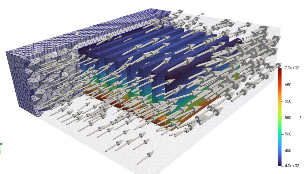
結果の確認