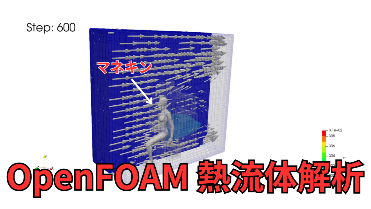
【第3回OpenFOAM熱流体解析】マネキン周りの熱流体解析(乱流モデル、ふく射モデル無し)
こんにちは(@t_kun_kamakiri)
本記事ではOpenFOAMを用いた熱流体解析の設定手順について解説を行います。
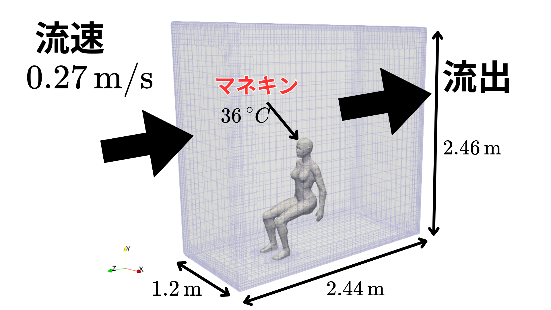
具体的には自然対流下でのマネキン周りの熱量を計算し、対流熱伝達と熱ふく射における影響度を調べることを目的とします。
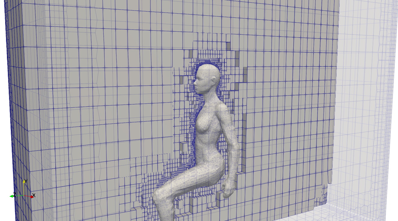
今回は、前回の記事で作成したメッシュ(snappyHexMesh)を用いて、マネキン周り熱流体解析を行う方法を紹介します。
マネキン周りの熱流体解析
- OpenFOAMを用いて流体解析を勉強している人
- OpenFOAMで熱流体解析(ふく射込み)を試したい人
本記事では本計算をするのではなく、まずはひな形を作るため、とりあえず計算できるところまでを行います。
そのため、
- メッシュはそこまでこだわらない(前回のまま)
- 乱流モデル無し
- ふく射モデル無し
とします。
OpenFOAM v2412(WSL Ubuntu 22.04)
フォルダ構成の確認
フォルダ構成は以下のようにしています。
|
1 2 3 4 5 |
kamakiri$ tree -L 1 . ├── cfMesh ├── model └── shm |
解析用フォルダを作成します。
|
1 2 |
mkdir run_shm_NoRad_base cd run_shm_NoRad_base |
次に、メッシュ情報ごとコピーします。
|
1 |
cp -r ../shm/* . |
メッシュ状態を念のため確認しておきます。
ParaViewを起動してpost.foam(空ファイル)を読みこむことで確認ができます。
解析設定
物性値
空気
- モル質量:$28.9\,\text{mol}/\text{g}$
- 定圧比熱:$1000\,\text{J}/\text{kg}\text{K}$
- 粘性係数:$1.73\times 10^{-5}\,\text{Pa}\cdot\text{s}$
- プラントル数:$0.7211$
理想気体として扱います。
|
1 2 3 4 5 6 7 8 9 10 11 12 13 14 15 16 17 18 19 20 21 22 23 24 25 26 27 28 29 30 |
thermoType { type heRhoThermo; mixture pureMixture; transport const; thermo hConst; equationOfState perfectGas; specie specie; energy sensibleEnthalpy; } pRef 100000; mixture { specie { molWeight 28.9; } thermodynamics { Cp 1006; Hf 0; } transport { mu 1.73e-05; Pr 0.7221; } } |
乱流モデル
乱流モデルは今回は使用しません。
次回以降で$k$-$\omega$SSTに設定する予定です。
simulationType laminar;としておくことで乱流モデルが使用されなくなります。
|
1 2 3 4 5 6 7 8 9 10 11 |
simulationType laminar; //simulationType RAS; RAS { RASModel kEpsilon; turbulence on; printCoeffs on; } |
ふく射モデル
ふく射モデルは今回使用しません。
次回以降でふく射モデルを設定します。
使用しているチュートリアルはfvDOMモデルのふく射設定ですが、
radiationModel none;//fvDOM;とすることでふく射を考慮しない設定になります。
ふく射モデルは以下のように6タイプあります。
|
1 2 |
Valid radiationModel types : 6(P1 fvDOM none opaqueSolid solarLoad viewFactor) |
|
1 2 3 4 5 6 7 8 9 10 11 12 13 14 15 16 17 18 19 20 21 22 23 24 25 26 27 |
radiation off;//on; radiationModel none;//fvDOM; fvDOMCoeffs { nPhi 3; nTheta 5; tolerance 1e-3; maxIter 10; } // Number of flow iterations per radiation iteration solverFreq 10; absorptionEmissionModel constantAbsorptionEmission; constantAbsorptionEmissionCoeffs { absorptivity absorptivity [ m^-1 ] 0.5; emissivity emissivity [ m^-1 ] 0.5; E E [ kg m^-1 s^-3 ] 0; } scatterModel none; sootModel none; |
放射率、吸収率、透過率などはconstant/boundaryRadiationPropertiesで設定しますが、こちらはふく射モデル用の設定ファイルなので今回は使用しません。
|
1 2 3 4 5 6 7 |
".*" { type lookup; emissivity 1.0; absorptivity 1.0; transmissivity 0.0; } |
境界条件
境界条件で使用するファイルは0/U, 0/T, 0/p_rgh, 0/pです。
p_rghは静圧から流体質量による圧力分を差し引いた量$p_{rgh}=p-rgh$なので、実際に設定が必要なのは0/U, 0/T, 0/p_rghです。
まずは流速の設定
|
1 2 3 4 5 6 7 8 9 10 11 12 13 14 15 16 17 18 19 20 21 22 23 24 25 26 27 28 29 30 31 32 33 34 35 36 37 38 39 40 |
dimensions [0 1 -1 0 0 0 0]; internalField uniform (0.0 0.0 -0.27); boundaryField { ".*" { type noSlip; } XMin { type noSlip; } XMax { type noSlip; } YMin { type noSlip; } YMax { type noSlip; } ZMin { type zeroGradient; } ZMax { type fixedValue; value uniform (0 0 -0.27); } } |
続いて温度の設定。
|
1 2 3 4 5 6 7 8 9 10 11 12 13 14 15 16 17 18 19 20 21 22 23 24 25 26 27 28 29 30 31 32 33 34 35 36 |
dimensions [0 0 0 1 0 0 0]; internalField uniform 298.15; boundaryField { ".*" { type fixedValue; value uniform 309.15; } XMin { type zeroGradient; } XMax { type zeroGradient; } YMin { type zeroGradient; } YMax { type zeroGradient; } ZMin { type zeroGradient; } ZMax { type zeroGradient; } } |
続いて圧力の設定。
|
1 2 3 4 5 6 7 8 9 10 11 12 13 14 15 16 17 18 19 20 21 22 23 24 25 26 27 28 29 30 31 32 33 34 35 36 37 38 39 40 41 42 |
dimensions [1 -1 -2 0 0 0 0]; internalField uniform 101325; boundaryField { ".*" { type fixedFluxPressure; value uniform 101325; } XMin { type fixedFluxPressure; value uniform 101325; } XMax { type fixedFluxPressure; value uniform 101325; } YMin { type fixedFluxPressure; value uniform 101325; } YMax { type fixedFluxPressure; value uniform 101325; } ZMin { type fixedValue; value uniform 101325.0; } ZMax { type fixedFluxPressure; value uniform 101325; } } |
圧力はp_rghから計算されるようにtype calculated;としておきます。
|
1 2 3 4 5 6 7 8 9 10 11 12 13 14 15 16 17 18 19 20 21 22 23 24 25 26 27 28 29 30 31 32 33 34 35 36 37 38 39 40 41 42 |
dimensions [1 -1 -2 0 0 0 0]; internalField uniform 101325.0; boundaryField { ".*" { type calculated; value uniform 101325.0; } XMin { type calculated; value uniform 101325.0; } XMax { type calculated; value uniform 101325.0; } YMin { type calculated; value uniform 101325.0; } YMax { type calculated; value uniform 101325.0; } ZMin { type calculated; value uniform 101325.0; } ZMax { type calculated; value uniform 101325.0; } } |
離散化スキーム
離散化スキームはチュートリアルをそのまま使用します。
対流項スキームは1次精度風上差分div(phi,U) bounded Gauss upwind; なので、数値的安定ではありますが、数値拡散をしやすいスキームです。
ラプラシアンのスキームはdefault Gauss linear corrected;非直交性考慮、非直交補正ありで設定されています。
|
1 2 3 4 5 6 7 8 9 10 11 12 13 14 15 16 17 18 19 20 21 22 23 24 25 26 27 28 29 30 31 32 33 34 35 36 37 38 39 40 41 42 |
ddtSchemes { default steadyState; } gradSchemes { default Gauss linear; } divSchemes { default none; div(phi,U) bounded Gauss upwind; energy bounded Gauss upwind; div(phi,K) $energy; div(phi,h) $energy; turbulence bounded Gauss upwind; div(phi,k) $turbulence; div(phi,epsilon) $turbulence; div(Ji,Ii_h) bounded Gauss linearUpwind grad(Ii_h); div(((rho*nuEff)*dev2(T(grad(U))))) Gauss linear; } laplacianSchemes { default Gauss linear corrected; } interpolationSchemes { default linear; } snGradSchemes { default corrected; } |
必要に応じて設定を変えると良いでしょう。
代数ソルバの設定
代数ソルバでは行列計算の設定、収束判定条件、不足緩和係数の設定を行います。
今回は収束判定の数値が大きすぎると、温度分布が定常になっていないのに残差は収束しきったとして計算が打ち切られてしまうことがあったので、residualControlの値は1桁(あるいは2桁)小さくしておきます。
|
1 2 3 4 5 6 7 8 9 10 11 12 13 14 15 16 17 18 19 20 21 22 23 24 25 26 27 28 29 30 31 32 33 34 35 36 37 38 39 40 41 42 43 44 45 46 47 48 49 50 51 52 53 54 55 56 57 58 59 60 61 62 63 64 |
solvers { p_rgh { solver PCG; preconditioner DIC; tolerance 1e-06; relTol 0.01; } Ii { solver GAMG; tolerance 1e-4; relTol 0; smoother symGaussSeidel; maxIter 5; nPostSweeps 1; } "(U|h|k|epsilon)" { solver PBiCGStab; preconditioner DILU; tolerance 1e-05; relTol 0.1; } } SIMPLE { nNonOrthogonalCorrectors 0; pRefCell 0; pRefValue 0; residualControl { p_rgh 1e-3; U 1e-4; h 1e-4; G 1e-4; // possibly check turbulence fields "(k|epsilon|omega)" 1e-4; "ILambda.*" 1e-4; } } relaxationFactors { fields { rho 1.0; p_rgh 0.7; } equations { U 0.2; h 0.2; k 0.5; epsilon 0.5; "ILambda.*" 0.7; } } |
計算制御の設定
タイムステップ数やfunction objectsの設定を行います。
タイムステップ数は定常になるまでを設定しておきます。
function objectsはいつも最低限以下を設定しています。
- 連続式の誤差
- 残差
- $y^{+}$
- 体積流量
|
1 2 3 4 5 6 7 8 9 10 11 12 13 14 15 16 17 18 19 20 21 22 23 24 25 26 27 28 29 30 31 32 33 34 35 36 37 38 39 40 41 42 43 44 45 46 47 48 49 50 51 52 53 54 55 56 57 58 59 60 61 62 63 64 65 66 67 68 69 70 71 72 73 74 75 76 77 78 79 80 81 82 83 84 85 86 87 88 89 90 91 92 93 94 95 96 97 98 99 100 101 102 103 104 105 106 107 108 109 110 111 112 113 114 115 116 117 118 119 120 121 122 123 124 125 126 127 128 129 130 131 132 133 134 135 136 137 138 139 140 141 142 143 144 145 146 147 |
application buoyantSimpleFoam; startFrom latestTime; startTime 0; stopAt endTime; endTime 2000; deltaT 1; writeControl timeStep; writeInterval 100; purgeWrite 0; writeFormat binary; writePrecision 6; writeCompression off; timeFormat general; timePrecision 6; runTimeModifiable true; functions { continuityError1 { type continuityError; libs ( fieldFunctionObjects ); // Mandatory entries (unmodifiable)// Optional entries (runtime modifiable) phi phi; // Optional (inherited) entries writePrecision 8; writeToFile yes; useUserTime yes; region region0; enabled yes; log yes; timeStart 0; timeEnd 6000; executeControl timeStep; executeInterval 1; writeControl timeStep; writeInterval 50; } residuals { type solverInfo; libs ( "libutilityFunctionObjects.so" ); fields ( ".*" ); } fieldMinMax1 { type fieldMinMax; libs ( fieldFunctionObjects ); // Mandatory entries (unmodifiable)// Mandatory entries (runtime modifiable) mode magnitude; fields ( U p T ); // Optional entries (runtime modifiable) location yes; writePrecision 8; writeToFile yes; useUserTime yes; region region0; enabled yes; log yes; timeStart 0; timeEnd 8000; executeControl timeStep; executeInterval 1; writeControl timeStep; writeInterval 100; } yPlus1 { type yPlus; libs ( fieldFunctionObjects ); // Mandatory entries (unmodifiable)// Optional (inherited) entries writePrecision 8; writeToFile yes; useUserTime yes; region region0; enabled yes; log yes; timeStart 0; timeEnd 8000; executeControl timeStep; executeInterval 1; writeControl timeStep; writeInterval 100; } ZMax { type surfaceFieldValue; libs ( "libfieldFunctionObjects.so" ); writeControl timeStep; log yes; writeFields no; regionType patch; name ZMax; operation sum; fields ( phi ); // Optional (inherited) entries writePrecision 8; writeToFile yes; useUserTime yes; region region0; enabled yes; timeStart 0; timeEnd 8000; executeControl timeStep; executeInterval 1; writeInterval 100; } ZMin { $ZMax; name ZMin; } } |
並列計算
チュートリアルに並列計算用の設定ファイルがない場合は適当なチュートリアルからコピーしてきます。
|
1 |
cp -r $FOAM_TUTORIALS/incompressible/icoFoam/cavityMappingTest/system/coarseMesh/decomposeParDict system/ |
$FOAM_TUTORIALS = /usr/lib/openfoam/openfoam2412/tutorials
今回は適当の4分割にして4並列で計算を実行します。
|
1 2 3 |
numberOfSubdomains 4; method scotch; |
計算実行
乱流モデルとふく射モデルは今回使用しないためファイルを一時避難させておきます。
|
1 2 |
mkdir -p 0/old mv 0/{G,IDefault,alphat,epsilon,k,nut} 0/old/ |
では、並列計算の実行します。
|
1 2 |
decomposePar mpirun -np 4 buoyantSimpleFoam -parallel > log.buoyantSimpleFoam & |
計算は数分で終わると思います。
結果の可視化
ParaViewで結果を確認します。
流出口で逆流しているように見えますね。
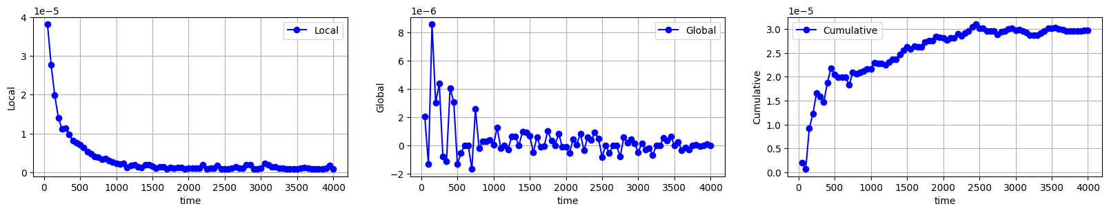
連続式の誤差や残差も見ておきます。
連続式の誤差
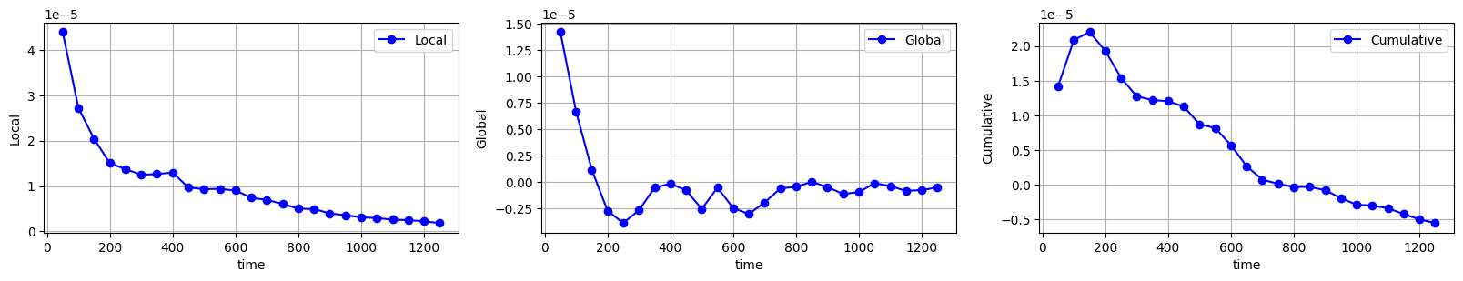 残差
残差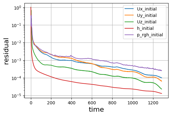 どちらもいい感じで収束しているように見えます。
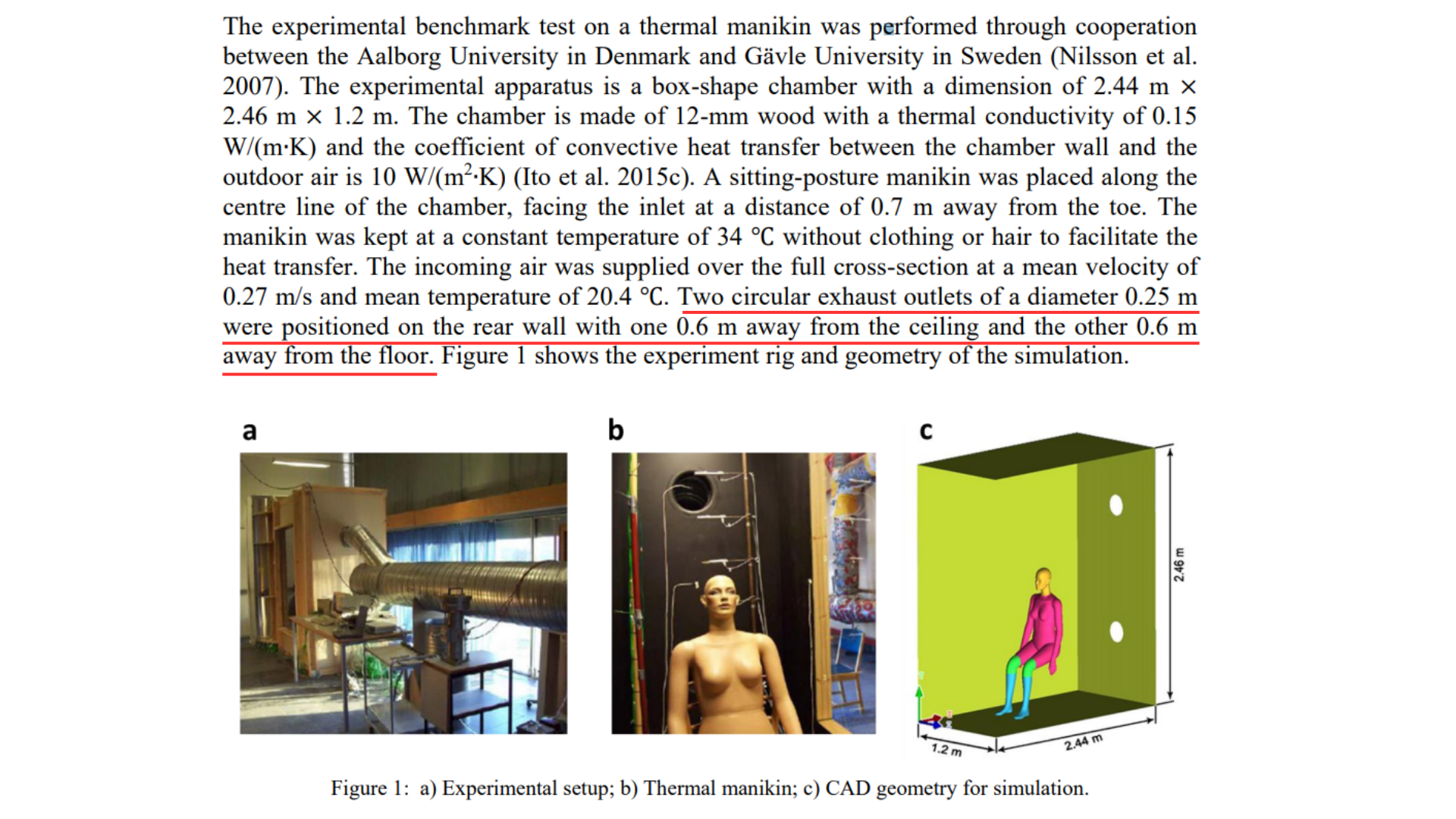
論文を確認すると流出口に排気口が必要だそうです。
ということでFreeCADに戻って外部領域のモデルを作り直しました。
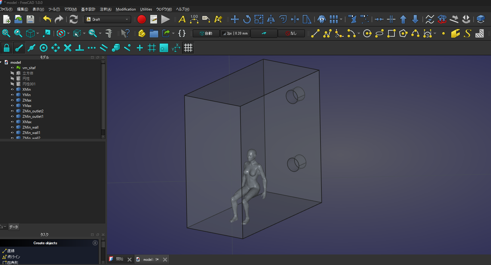 排気口を設けた解析で再度計算した結果がこちら。
 連続式の誤差
 残差
残差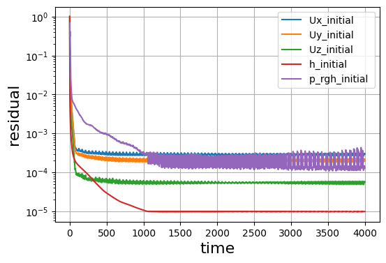
温度分布も安定しており、連続式の誤差や残差が収束していますね。
まとめ
本記事ではOpenFOAMを用いた熱流体解析の準備としてマネキンモデルまわりの熱流体解析を行いました。
今回は乱流モデル設定なし、ふく射モデルの設定なしで解析を行いましたが、今後は乱流モデルやふく射モデルを追加し、より実際の環境に近い条件での解析を行う予定です。結果の可視化や温度分布の比較も進めていきます。
次回は、排気口を取り付けたモデルを用いて、乱流モデルの設定$k$-$\omega$SSTをした解析を行います。
計算力学技術者のための問題アプリ
計算力学技術者熱流体2級、1級対策アプリをリリースしました。
- 下記をクリックしてホームページでダウンロードできます。
- LINE公式に登録すると無料で問題の一部を閲覧できます。
※LINEの仕様で数式がずれていますが、アプリでは問題ありません。
- 計算力学技術者の熱流体2級問題アプリ作成
リリース後も試行錯誤をしながら改善に努め日々アップデートしています。
備忘録として作成の過程を綴っています。
OpenFOAMに関する技術書を販売中!
OpenFOAMを自宅で学べるシリーズを販売中です。
OpenFOAM初学者から中級者向けの技術書となっていますので、ぜひよろしくお願いいたします。
次回の技術書典18に向けて内容を考え中です。
乞うご期待!!
お勧めの参考書
本記事の内容について触れている書籍がこちらです。
CFD(流体解析)のガイドブックというタイトルだけあって、熱流体に関する内容は網羅的に書かれています。
乱流モデルの数式の展開が非常に丁寧なのはこちらの参考書です。
今まで読んだ本の中で途中式もしっかり書いてあって一番丁寧でした。
乱流モデルの話だけでなく、混相流(気液、固液)や粒子法、浅水方程式の話も乗っているので重宝しています。
乱流モデルはこちらもお勧めです。
前半は数値シミュレーションの離散化の話で、後半に乱流モデルの話が出てきます。
乱流モデルのざっくりした解説と流体全般の基礎知識にはこちらがちょうど良いでしょう。